Class: `Image`¶

class pykitPIV.image.ImageSpecs(n_images=1, size=(512, 512), size_buffer=10, random_seed=None, exposures=(0.5, 1), maximum_intensity=65535, laser_beam_thickness=1, laser_over_exposure=1, laser_beam_shape=0.95, no_laser_plane=False, alpha=0.125, extend_gaussian=1, covariance_matrix=None, clip_intensities=True, normalize_intensities=False, dtype=<class 'numpy.float64'>)¶

Configuration object for the Image class.

Example:

from pykitPIV import ImageSpecs

# Instantiate an object of ImageSpecs class:
image_spec = ImageSpecs()

# Change one field of motion_spec:
image_spec.exposures = 0.95

# You can print the current values of all attributes:
print(image_spec)

class pykitPIV.image.Image(verbose=False, dtype=<class 'numpy.float64'>, random_seed=None)¶

Stores and plots synthetic PIV images and/or the associated flow targets at any stage of particle generation and movement.

Example:

from pykitPIV import Image
import numpy as np

# Initialize an image object:
image = Image(verbose=False,
              dtype=np.float32,
              random_seed=100)

Parameters:

verbose – (optional) bool specifying if the verbose print statements should be displayed.
dtype – (optional) numpy.dtype specifying the data type for image intensities. To reduce memory, you can switch from the default numpy.float64 to numpy.float32.
random_seed – (optional) int specifying the random seed for random number generation in numpy. If specified, all operations are reproducible.

Attributes:

verbose - (read-only) as per user input.
dtype - (read-only) as per user input.
random_seed - (read-only) as per user input.
images_I1 - (read-only) numpy.ndarray of size \((N, C_{in}, H+2b, W+2b)\), where \(N\) is the number PIV image pairs, \(C_{in}\) is the number of channels (one channel, greyscale, is supported at the moment), \(H\) is the height and \(W\) is the width of each PIV image, \(I_1\), and \(b\) is the optional buffer. Only available after Image.add_particles() has been called.
images_I2 - (read-only) numpy.ndarray of size \((N, C_{in}, H+2b, W+2b)\), where \(N\) is the number PIV image pairs, \(C_{in}\) is the number of channels (one channel, greyscale, is supported at the moment), \(H\) is the height and \(W\) is the width of each PIV image, \(I_2\), and \(b\) is the optional buffer. Only available after Image.add_motion() has been called.
exposures_per_image - (read-only) numpy.ndarray specifying the template for the light exposure for each image. Only available after Image.add_reflected_light has been called.
maximum_intensity - (read-only) int specifying the maximum intensity that was used when adding reflected light to the image. Only available after Image.add_reflected_light has been called.

pykitPIV.image.Image.add_particles(self, particles)¶

Adds particles to the image. Particles should be defined using the Particle class.

Calling this function populates the image.images_I1 attribute and the private attribute image.__particles which gives the user access to attributes from the Particle object.

Example:

from pykitPIV import Particle, Image

# Initialize a particle object:
particles = Particle(1,
                     size=(128, 512),
                     size_buffer=10,
                     random_seed=100)

# Initialize an image object:
image = Image(random_seed=100)

# Add particles to an image:
image.add_particles(particles)

Parameters:: particles – Particle class instance specifying the properties and positions of particles.

pykitPIV.image.Image.add_flowfield(self, flowfield)¶

Adds the flow field to the image. The flow field should be defined using the FlowField class.

Calling this function populates the private attribute image.__flowfield which gives the user access to attributes from the FlowField object.

Example:

from pykitPIV import FlowField, Image

# Initialize a flow field object:
flowfield = FlowField(1,
                      size=(128, 512),
                      size_buffer=10,
                      time_separation=1,
                      random_seed=100)

# Initialize an image object:
image = Image(random_seed=100)

# Add flow field to an image:
image.add_flowfield(flowfield)

Parameters:: flowfield – FlowField class instance specifying the flow field.

pykitPIV.image.Image.add_motion(self, motion)¶

Adds particle movement to the image. The movement should be defined using the Motion class.

Calling this function populates the private attribute image.__motion which gives the user access to attributes from the Motion object.

Example:

from pykitPIV import Particle, FlowField, Motion, Image

# Initialize a particle object:
particles = Particle(1,
                     size=(128, 512),
                     size_buffer=10,
                     random_seed=100)

# Initialize a flow field object:
flowfield = FlowField(1,
                      size=(128, 512),
                      size_buffer=10,
                      time_separation=1,
                      random_seed=100)

# Initialize a motion object:
motion = Motion(particles, flowfield)

# Initialize an image object:
image = Image(random_seed=100)

# Add motion to an image:
image.add_motion(motion)

Parameters:: motion – Motion class instance specifying the movement of particles from one instance in time to the next. In general, the movement is defined by the FlowField class applied to particles defined by the Particle class.

pykitPIV.image.Image.get_velocity_field(self)¶

Returns the velocity field from the object of the FlowField class.

Example:

from pykitPIV import Particle, FlowField, Image

# Initialize a particle object:
particles = Particle(1,
                     size=(128, 512),
                     size_buffer=10,
                     random_seed=100)

# Initialize a flow field object:
flowfield = FlowField(1,
                      size=(128, 512),
                      size_buffer=10,
                      time_separation=1,
                      random_seed=100)

# Generate random velocity field:
flowfield.generate_random_velocity_field(displacement=(0, 10),
                                         gaussian_filters=(10, 30),
                                         n_gaussian_filter_iter=6)

# Initialize an image object:
image = Image(random_seed=100)

# Add flow field to an image:
image.add_flowfield(flowfield)

# Access the velocity field:
V = image.get_velocity_field()

Returns:

velocity_field - as per FlowField class.

pykitPIV.image.Image.get_velocity_field_magnitude(self)¶

Returns the velocity field magnitude from the object of the FlowField class.

Example:

from pykitPIV import Particle, FlowField, Image

# Initialize a particle object:
particles = Particle(1,
                     size=(128, 512),
                     size_buffer=10,
                     random_seed=100)

# Initialize a flow field object:
flowfield = FlowField(1,
                      size=(128, 512),
                      size_buffer=10,
                      time_separation=1,
                      random_seed=100)

# Generate random velocity field:
flowfield.generate_random_velocity_field(displacement=(0, 10),
                                         gaussian_filters=(10, 30),
                                         n_gaussian_filter_iter=6)

# Initialize an image object:
image = Image(random_seed=100)

# Add flow field to an image:
image.add_flowfield(flowfield)

# Access the velocity field magnitude:
V_mag = image.get_velocity_field_magnitude()

Returns:

velocity_field_magnitude - as per FlowField class.

pykitPIV.image.Image.get_displacement_field(self)¶

Returns the displacement field from the object of the FlowField class.

Example:

from pykitPIV import FlowField, Image

# Initialize a flow field object:
flowfield = FlowField(1,
                      size=(128, 512),
                      size_buffer=10,
                      time_separation=0.1,
                      random_seed=100)

# Generate random velocity field:
flowfield.generate_random_velocity_field(displacement=(0, 10),
                                         gaussian_filters=(10, 30),
                                         n_gaussian_filter_iter=6)

# Initialize an image object:
image = Image(random_seed=100)

# Add motion to an image:
image.add_flowfield(flowfield)

# Access the displacement field:
ds = image.get_displacement_field()

Returns:

displacement_field - as per FlowField class.

pykitPIV.image.Image.get_displacement_field_magnitude(self)¶

Returns the displacement field magnitude from the object of the FlowField class.

Example:

from pykitPIV import FlowField, Image

# Initialize a flow field object:
flowfield = FlowField(1,
                      size=(128, 512),
                      size_buffer=10,
                      time_separation=0.1,
                      random_seed=100)

# Generate random velocity field:
flowfield.generate_random_velocity_field(displacement=(0, 10),
                                         gaussian_filters=(10, 30),
                                         n_gaussian_filter_iter=6)

# Initialize an image object:
image = Image(random_seed=100)

# Add motion to an image:
image.add_flowfield(flowfield)

# Access the displacement field magnitude:
ds_mag = image.get_displacement_field_magnitude()

Returns:

displacement_field_magnitude - as per FlowField class.

pykitPIV.image.Image.compute_light_intensity_at_pixel(self, peak_intensity, particle_diameter, coordinate_height, coordinate_width, alpha=0.125, covariance_matrix=None)¶

Computes the intensity of light reflected from a particle at a requested pixel at position relative to the particle centroid.

The reflected light follows a Gaussian distribution which can be either univariate (in which case particles are spherical Gaussians) or covariate (in which case particles have an elongated shape).

For a univariate distrubution, the light intensity value, \(i_p\), at the requested pixel, \(p\), is computed as:

\[i_p = i_{\text{peak}} \cdot \exp \Big(- \frac{h_p^2 + w_p^2}{\alpha \cdot d_p^2} \Big)\]

where:

\(i_{\text{peak}}\) is the peak intensity applied at the particle centroid.
\(h_p\) is the pixel coordinate in the image height direction relative to the particle centroid.
\(w_p\) is the pixel coordinate in the image width direction relative to the particle centroid.
\(\alpha\) is a custom multiplier, \(\alpha\). The default value is \(\alpha = 1/8\).
\(d_p\) is the particle diameter.

For a covariate distrubution, the light intensity value, \(i_p\), at the requested pixel, \(p\), is computed as:

\[i_p = i_{\text{peak}} \cdot \exp \Big(- \frac{\mathbf{r} \cdot \mathbf{C}^{-1} \cdot \mathbf{r}^{\top}}{\alpha \cdot d_p^2} \Big)\]

where:

\(\mathbf{C}\) is the covariance matrix that is positive semi-definite and \(\mathbf{C}^{-1}\) is its inverse.
\(\mathbf{r}\) is the position vector, \(\mathbf{r} = [w_p, h_p]\).

Parameters:

peak_intensity – float specifying the peak intensity, \(i_{\text{peak}}\), to apply at the particle centroid.
particle_diameter – float specifying the particle diameter \(d_p\).
coordinate_height – float specifying the pixel coordinate in the image height direction, \(h_p\), relative to the particle centroid.
coordinate_width – float specifying the pixel coordinate in the image width direction, \(w_p\), relative to the particle centroid.
alpha – (optional): float specifying the custom multiplier, \(\alpha\), for the squared particle radius. The default and recommended value is \(1/8\) as per Raffel et al. (2018), Rabault et al. (2017) and Manickathan et al. (2022).
covariance_matrix – (optional): numpy.ndarray specifying the covariance matrix that has to be positive semi-definite. If set to None, the particle images will be generated from a univariate distrubtion (as spherical Gaussians). It has to have size (2, 2).

Returns:

pixel_value - float specifying the light intensity value at the requested pixel.

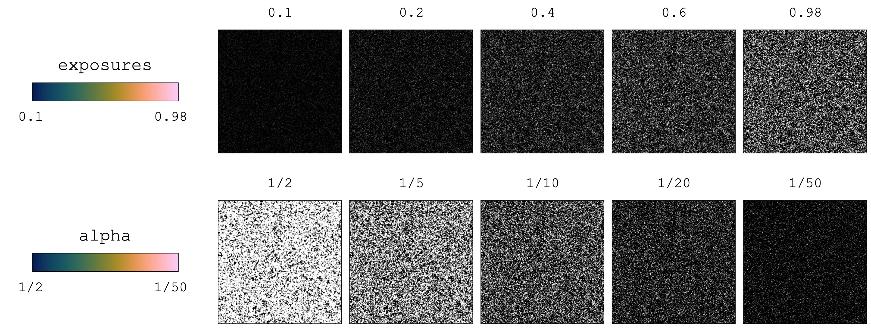
pykitPIV.image.Image.add_reflected_light(self, exposures=(0.5, 1), maximum_intensity=65535, laser_beam_thickness=2, laser_over_exposure=1, laser_beam_shape=0.85, no_laser_plane=False, alpha=0.125, extend_gaussian=1, covariance_matrix=None, clip_intensities=True, normalize_intensities=False)¶

Creates particle shapes and adds laser light reflected from particles.

The reflected light follows a Gaussian distribution and is computed using the Image.compute_light_intensity_at_pixel() method.

The particle shapes can be spherical Gaussians or can have a non-zero covariance. In the latter case, the user has to provide a full covariance matrix that is positive semi-definite.

Example:

from pykitPIV import Particle, Image

# Initialize a particle object:
particles = Particle(1,
                     size=(128, 512),
                     size_buffer=10)

# Initialize an image object:
image = Image(random_seed=100)

# Add particles to an image:
image.add_particles(particles)

# Add reflected light to an image:
image.add_reflected_light(exposures=(0.5, 0.9),
                          maximum_intensity=2**16-1,
                          laser_beam_thickness=1,
                          laser_over_exposure=1,
                          laser_beam_shape=0.95,
                          no_laser_plane=False,
                          alpha=1/8,
                          extend_gaussian=1,
                          covariance_matrix=None,
                          clip_intensities=True,
                          normalize_intensities=False)

Alternatively, we can model astigmatic PIV by providing a coviariance matrix:

Example:

# Define a full, positive semi-definite covariance matrix:
covariance_matrix = np.array([[3.0, -2],
                              [-2, 2.0]])

# Add reflected light to an image:
image.add_reflected_light(exposures=(0.5, 0.9),
                          maximum_intensity=2**16-1,
                          laser_beam_thickness=1,
                          laser_over_exposure=1,
                          laser_beam_shape=0.95,
                          no_laser_plane=False,
                          alpha=1/8,
                          extend_gaussian=1,
                          covariance_matrix=covariance_matrix,
                          clip_intensities=True,
                          normalize_intensities=False)

Parameters:

exposures – (optional) tuple of two numerical elements specifying the minimum (first element) and maximum (second element) light exposure. It can also be set to int or float to generate a fixed exposure value across all \(N\) image pairs.
maximum_intensity – (optional) int specifying the maximum light intensity. This will be the brightest possible pixel, which will only happen if the particle is located at the center of that pixel and at the center of the laser plane. All particles with an offset with respect to the laser plane will have a lower intensity than the maximum.
laser_beam_thickness – (optional) int or float specifying the thickness of the laser beam. With a small thickness, particles that are even slightly off-plane will appear darker. Note, that the thicker the laser plane, the larger the distance that the particle can travel away from the laser plane to lose its luminosity.
laser_over_exposure – (optional) int or float specifying the overexposure of the laser beam.
laser_beam_shape – (optional) int or float specifying the spread of the Gaussian shape of the laser beam. The larger this number is, the wider the Gaussian light distribution from the laser and more particles will be illuminated.
no_laser_plane – (optional) bool specifying whether the laser plane is used to illuminate particles. For PIV images, set to False. For BOS images set to True.
alpha –
(optional): float specifying the custom multiplier, \(\alpha\), for the squared particle radius as per the Particle.compute_light_intensity_at_pixel() method. The default and recommended value is \(1/8\) as per Raffel et al. (2018), Rabault et al. (2017) and Manickathan et al. (2022).
extend_gaussian – (optional): int specifying the multiple of the particle radius to be filled with the Gaussian blur. For BOS images, it is recommended to increase this number to, say, 2. For PIV images, it can be equal to 1. Note that a higher number will increase the computation time for adding light intensity to images.
covariance_matrix – (optional): numpy.ndarray specifying the covariance matrix that has to be positive semi-definite. If set to None, the particle images will be generated from a univariate distrubtion (as spherical Gaussians). It has to have size (2, 2).
clip_intensities – (optional): bool specifying whether the image intensities should be clipped if any pixel exceeds the maximum light intensity. Only one of clip_intensities, normalize_intensities can be True.
normalize_intensities – (optional): bool specifying whether the image intensities should be normalized if any pixel exceeds the maximum light intensity. Only one of clip_intensities, normalize_intensities can be True.

pykitPIV.image.Image.warp_images(self, time_separation=1, order=1, mode='constant')¶

Warps images according to the velocity field. This function can be used to produce \(I_2\) in background-oriented Schlieren (BOS) by warping \(I_1\).

Note

This function uses scipy.ndimage.map_coordinates to warp images.

Example:

from pykitPIV import Particle, FlowField, Image

# We are going to generate 10 BOS image pairs:
n_images = 10

# Specify size in pixels for each image:
image_size = (512, 512)

# Initialize a particle object:
particles = Particle(n_images,
                     size=image_size,
                     size_buffer=10,
                     diameters=10,
                     distances=1,
                     densities=1.2,
                     diameter_std=0,
                     seeding_mode='poisson',
                     random_seed=100)

# Initialize an image object:
image = Image(random_seed=100)
image.add_particles(particles)

image.add_reflected_light(exposures=0.99,
                          maximum_intensity=2**16-1,
                          no_laser_plane=True,
                          alpha=1/8,
                          extend_gaussian=2)

# Initialize a flow field object:
flowfield = FlowField(n_images,
                      size=image_size,
                      size_buffer=10,
                      time_separation=1,
                      random_seed=100)

flowfield.generate_potential_velocity_field(imposed_origin=None,
                                            displacement=(2, 2))


image.add_flowfield(flowfield)

# Warp images:
image.warp_images(time_separation=10)

Parameters:

time_separation – float or int specifying the time separation, \(\Delta t\), that will scale the velocity field to obtain a displacement field.
order – int specifying the order of the spline interpolation as per scipy.ndimage.map_coordinates. It has to be a number between 0 and 5.
mode – str specifying how the input array is extended beyond its boundaries. With sufficient buffer size this should not affect the proper image area.

pykitPIV.image.Image.remove_buffers(self, input_tensor)¶

Removes image buffers from the input tensor. If the input tensor is a four-dimensional array of size \((N, \_, H+2b, W+2b)\), then the output is a four-dimensional tensor array of size \((N, \_, H, W)\).

Example:

from pykitPIV import Particle, Image

# Initialize a particle object:
particles = Particle(10,
                     size=(128, 512),
                     size_buffer=10)

# Initialize an image object:
image = Image(random_seed=100)

# Add particles to an image:
image.add_particles(particles)

# Add reflected light to an image:
image.add_reflected_light(exposures=(0.5, 0.9),
                          maximum_intensity=2**16-1,
                          laser_beam_thickness=1,
                          laser_over_exposure=1,
                          laser_beam_shape=0.95,
                          alpha=1/8,
                          covariance_matrix=None,
                          clip_intensities=True,
                          normalize_intensities=False)

# Remove buffers from the first image frame:
images_I1 = image.remove_buffers(image.images_I1)

Parameters:

input_tensor – numpy.ndarray specifying the input tensor. It has to have size \((N, C_{in}, H+2b, W+2b)\).

Returns:

input_tensor - numpy.ndarray specifying the input tensor with buffers removed. It has size \((N, C_{in}, H, W)\).

pykitPIV.image.Image.measure_counts(self, image)¶

Measures the number of light intensity counts in a given image.

Example:

from pykitPIV import Particle, Image

# Initialize a particle object:
particles = Particle(10,
                     size=(20, 20),
                     size_buffer=0)

# Initialize an image object:
image = Image(random_seed=100)

# Add particles to an image:
image.add_particles(particles)

# Add reflected light to an image:
image.add_reflected_light(exposures=(0.5, 0.9),
                          maximum_intensity=2**16-1,
                          laser_beam_thickness=1,
                          laser_over_exposure=1,
                          laser_beam_shape=0.95,
                          alpha=1/8,
                          covariance_matrix=None,
                          clip_intensities=True,
                          normalize_intensities=False)

# Measure light intensity counts:
counts_dictionary = image.measure_counts(image.images_I1[0,:,:])

Parameters:

image – numpy.ndarray specifying the single PIV image.

Returns:

counts_dictionary - dict specifying the measured counts. Keys are pixel intensities and values are the number of occurrence of the given intensity in the image.

pykitPIV.image.Image.concatenate_tensors(self, input_tensor_tuple)¶

Concatenates multiple four-dimensional tensor arrays along the second dimension (the “channel” dimension).

Example:

from pykitPIV import Particle, FlowField, Motion, Image

# Initialize a particle object:
particles = Particle(1,
                     size=(128, 512),
                     size_buffer=10,
                     random_seed=100)

# Initialize a flow field object:
flowfield = FlowField(1,
                      size=(128, 512),
                      size_buffer=10,
                      time_separation=1,
                      random_seed=100)

# Generate random velocity field:
flowfield.generate_random_velocity_field(displacement=(0, 10),
                                         gaussian_filters=(10, 30),
                                         n_gaussian_filter_iter=6)

# Initialize a motion object:
motion = Motion(particles, flowfield)
motion.runge_kutta_4th(n_steps=10)

# Initialize an image object:
image = Image(random_seed=100)

# Add motion to an image:
image.add_motion(motion)

# Add particles to an image:
image.add_particles(particles)

# Add light reflected from particles:
image.add_reflected_light(exposures=(0.6, 0.65),
                          maximum_intensity=2**16-1,
                          laser_beam_thickness=1,
                          laser_over_exposure=1,
                          laser_beam_shape=0.95,
                          alpha=1/10)

# Concatenate image frames:
I = image.concatenate_tensors((image.images_I1,
                               image.images_I2))

Returns:

input_tensor_tuple - tuple of numpy.ndarray specifying the four-dimensional tensors to concatenate. Each numpy.ndarray should have size \((N, \_, H, W)\), where \(N\) is the number of PIV image pairs, \(H\) is the height and \(W\) is the width of each PIV image. The second dimension refers to items being concatenated.

pykitPIV.image.Image.save_to_tiff(self, image_tensor, filename=None, verbose=False)¶

Saves the image pairs tensor to individual .tiff images.

Example:

from pykitPIV import Particle, FlowField, Motion, Image

# We are going to generate 4 PIV image pairs:
n_images = 4

# Specify size in pixels for each image:
image_size = (256, 256)

# Initialize a particle object:
particles = Particle(n_images=n_images,
                     size=image_size,
                     size_buffer=10,
                     diameters=(2, 4),
                     distances=(1, 2),
                     densities=(0.01, 0.05),
                     diameter_std=(0.1, 1),
                     seeding_mode='random',
                     random_seed=100)

# Initialize a flow field object:
flowfield = FlowField(n_images=n_images,
                      size=image_size,
                      size_buffer=10,
                      time_separation=1,
                      random_seed=100)

# Generate random velocity field:
flowfield.generate_random_velocity_field(gaussian_filters=(2, 10),
                                         n_gaussian_filter_iter=10,
                                         displacement=(2, 5))

# Initialize a motion object:
motion = Motion(particles,
                flowfield,
                particle_loss=(0, 2),
                particle_gain='matching',
                verbose=False,
                random_seed=None)

# Advect particles:
motion.forward_euler(n_steps=10)

# Initialize an image object:
image = Image(random_seed=100)

# Add particles to an image:
image.add_particles(particles)

# Add flow field to an image:
image.add_flowfield(flowfield)

# Add motion to an image:
image.add_motion(motion)

# Add reflected light to an image:
image.add_reflected_light(exposures=(0.5, 0.9),
                          maximum_intensity=2**16-1,
                          laser_beam_thickness=1,
                          laser_over_exposure=1,
                          laser_beam_shape=0.95,
                          alpha=1/8,
                          covariance_matrix=None,
                          clip_intensities=True,
                          normalize_intensities=False)

# Remove buffers from images:
images_I1 = image.remove_buffers(image.images_I1)
images_I2 = image.remove_buffers(image.images_I2)

# Prepare an image pairs tensor to save:
images_intensities = image.concatenate_tensors((images_I1, images_I2))

# Save images to .tiff:
image.save_to_tiff(images_intensities,
                   filename='dataset',
                   verbose=True)

Parameters:

image_tensor – numpy.ndarray specifying the image pairs tensor to save. It should be of size \((N, 2, H, W)\).
filename – (optional) str specifying the path and filename to save the .tiff images. Note that '-#-I1' or '-#-I2' will be added automatically to your filename for each saved image. If set to None, a default name 'PIV-dataset-#-I1.tiff' or 'PIV-dataset-#-I2.tiff' will be used.
verbose – (optional) bool for printing verbose details.

pykitPIV.image.Image.save_to_h5(self, tensors_dictionary, save_individually=False, filename=None, verbose=False)¶

Saves the image pairs tensor and/or the associated flow targets tensor to .h5 data format.

Example:

from pykitPIV import Particle, FlowField, Motion, Image

# We are going to generate 10 PIV image pairs:
n_images = 10

# Specify size in pixels for each image:
image_size = (128, 512)

# Initialize a particle object:
particles = Particle(n_images=n_images,
                     size=image_size,
                     size_buffer=10,
                     diameters=(2, 4),
                     distances=(1, 2),
                     densities=(0.01, 0.05),
                     diameter_std=(0.1, 1),
                     seeding_mode='random',
                     random_seed=100)

# Initialize a flow field object:
flowfield = FlowField(n_images=n_images,
                      size=image_size,
                      size_buffer=10,
                      time_separation=1,
                      random_seed=100)

# Generate random velocity field:
flowfield.generate_random_velocity_field(gaussian_filters=(2, 10),
                                         n_gaussian_filter_iter=10,
                                         displacement=(2, 5))

# Initialize a motion object:
motion = Motion(particles,
                flowfield,
                particle_loss=(0, 2),
                particle_gain='matching',
                verbose=False,
                random_seed=None)

# Advect particles:
motion.forward_euler(n_steps=10)

# Initialize an image object:
image = Image(random_seed=100)

# Add particles to an image:
image.add_particles(particles)

# Add flow field to an image:
image.add_flowfield(flowfield)

# Add motion to an image:
image.add_motion(motion)

# Add reflected light to an image:
image.add_reflected_light(exposures=(0.5, 0.9),
                          maximum_intensity=2**16-1,
                          laser_beam_thickness=1,
                          laser_over_exposure=1,
                          laser_beam_shape=0.95,
                          alpha=1/8,
                          covariance_matrix=None,
                          clip_intensities=True,
                          normalize_intensities=False)

# Remove buffers from images:
images_I1 = image.remove_buffers(image.images_I1)
images_I2 = image.remove_buffers(image.images_I2)

# Remove buffers from targets:
velocity_field = image.remove_buffers(image.get_velocity_field())
displacement_field = image.remove_buffers(image.get_displacement_field())

# Prepare a tensors dictionary to save:
images_intensities = image.concatenate_tensors((images_I1, images_I2))
flow_targets = image.concatenate_tensors((velocity_field, displacement_field))

tensors_dictionary = {"I"      : images_intensities,
                      "target" : flow_targets}

# Save tensors to h5:
image.save_to_h5(tensors_dictionary,
                 save_individually=False,
                 filename='dataset.h5',
                 verbose=True)

Parameters:

tensors_dictionary – dict specifying the tensors to save.
save_individually – (optional) bool specifying if each image pair and the associated targets should be saved to a separate file. It is recommended to save individually for large datasets that will be uploaded by PyTorch, since at any iteration of a machine learning algorithm, only a small batch of samples is uploaded to memory.
filename – (optional) str specifying the path and filename to save the .h5 data. Note that '-pair-#' will be added automatically to your filename for each saved image pair. If set to None, a default name 'PIV-dataset-pair-#.h5' will be used.
verbose – (optional) bool for printing verbose details.

pykitPIV.image.Image.upload_from_h5(self, filename=None)¶

Upload image pairs tensor and/or the associated flow targets tensor from .h5 data format.

Example:

from pykitPIV import Image

# Instantiate an empty image object:
image = Image()

# Upload the saved dataset to the empty image object:
tensors_dictionary_uploaded = image.upload_from_h5(filename='dataset.h5')

Parameters:

filename – (optional) str specifying the path and filename to save the .h5 data. Note that '-pair-#' will be added automatically to your filename for each saved image pair. If set to None, a default name 'PIV-dataset-pair-#.h5' will be used.

Returns:

tensors_dictionary - dict specifying the dataset tensors.

pykitPIV.image.Image.plot(self, idx, instance=1, with_buffer=False, xlabel=None, ylabel=None, xticks=True, yticks=True, title=None, cmap='Greys_r', cbar=False, origin='lower', figsize=(5, 5), dpi=300, filename=None)¶

Plots a single, static PIV image, \(I_1\) or \(I_2\).

Parameters:

idx – int specifying the index of the image to plot out of n_images number of images.
instance – (optional) int specifying whether \(I_1\) (instance=1) or \(I_2\) (instance=2) should be plotted.
with_buffer – (optional) bool specifying whether the buffer for the image size should be visualized. If set to False, the true PIV image size is visualized. If set to True, the PIV image with a buffer is visualized and buffer outline is marked with a red rectangle.
xlabel – (optional) str specifying \(x\)-label.
ylabel – (optional) str specifying \(y\)-label.
xticks – (optional) bool specifying if ticks along the \(x\)-axis should be plotted.
yticks – (optional) bool specifying if ticks along the \(y\)-axis should be plotted.
title – (optional) str specifying figure title.
cmap – (optional) str or an object of matplotlib.colors.ListedColormap specifying the color map to use.
cbar – (optional) bool specifying whether colorbar should be plotted.
origin – (optional) str specifying the origin location. It can be 'upper' or 'lower'.
figsize – (optional) tuple of two numerical elements specifying the figure size as per matplotlib.pyplot.
dpi – (optional) int specifying the dpi for the image.
filename – (optional) str specifying the path and filename to save an image. If set to None, the image will not be saved.

Returns:

plt - matplotlib.pyplot image handle.

pykitPIV.image.Image.plot_image_pair(self, idx, with_buffer=False, xlabel=None, ylabel=None, xticks=True, yticks=True, title=None, cmap='Greys_r', cbar=False, origin='lower', figsize=(5, 5), dpi=300, filename=None)¶

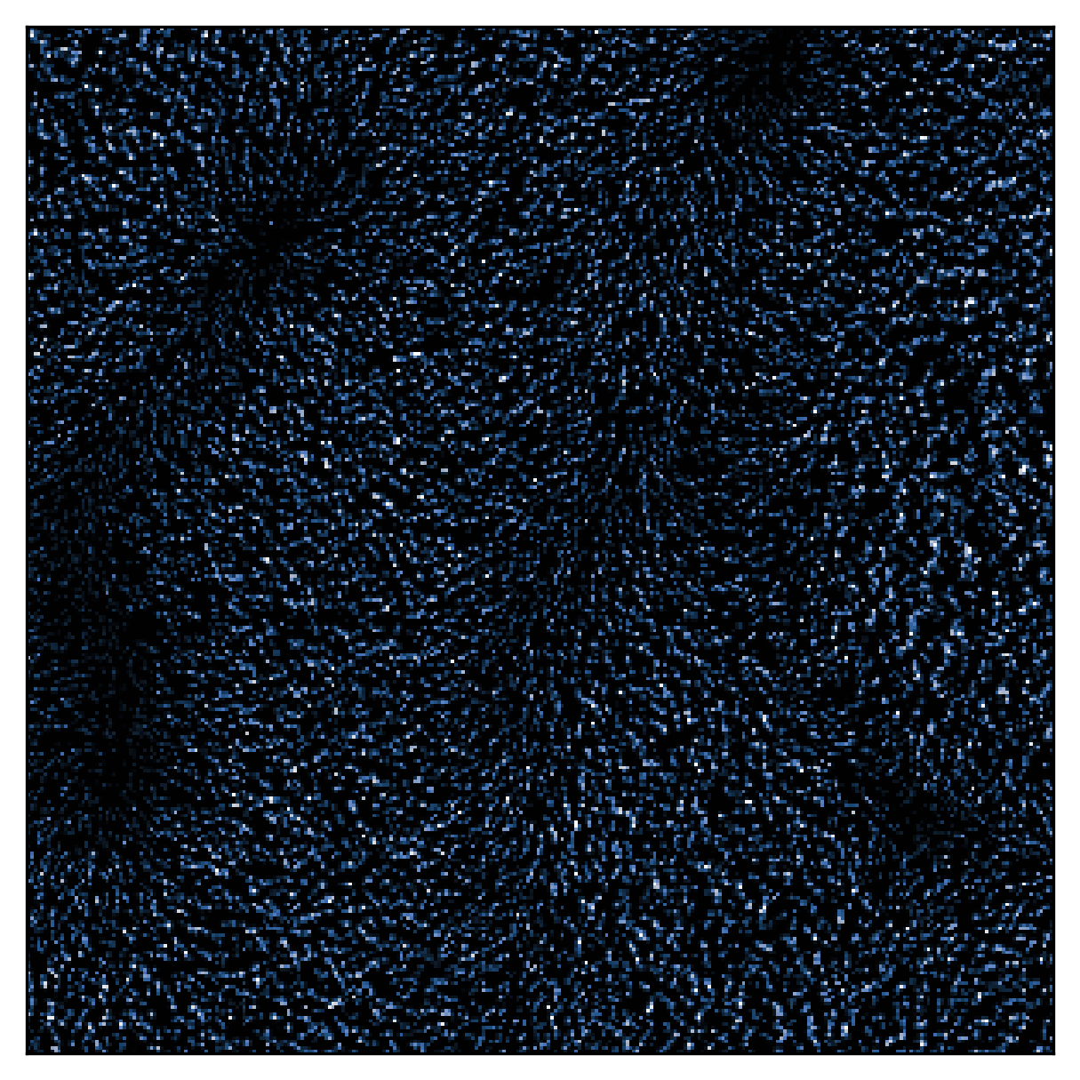
Plots a PIV image pair on single, static PIV image by superimposing \(I_1 - I_2\).

Example:

Given the following velocity field magnitude:

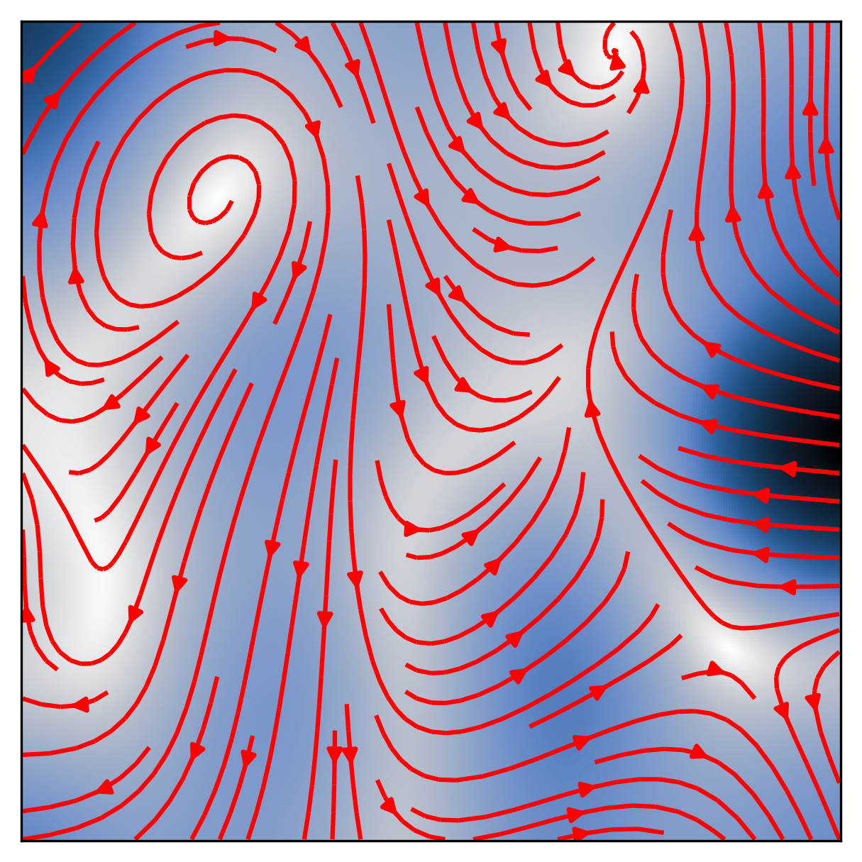
../_images/Image_plot_velocity_field_magnitude.png

This function will produce the following image:

Parameters:

idx – int specifying the index of the image to plot out of n_images number of images.
with_buffer – (optional) bool specifying whether the buffer for the image size should be visualized. If set to False, the true PIV image size is visualized. If set to True, the PIV image with a buffer is visualized and buffer outline is marked with a red rectangle.
xlabel – (optional) str specifying \(x\)-label.
ylabel – (optional) str specifying \(y\)-label.
xticks – (optional) bool specifying if ticks along the \(x\)-axis should be plotted.
yticks – (optional) bool specifying if ticks along the \(y\)-axis should be plotted.
title – (optional) str specifying figure title.
cmap –
(optional) str or an object of matplotlib.colors.ListedColormap specifying the color map to use.
cbar – (optional) bool specifying whether colorbar should be plotted.
origin – (optional) str specifying the origin location. It can be 'upper' or 'lower'.
figsize – (optional) tuple of two numerical elements specifying the figure size as per matplotlib.pyplot.
dpi – (optional) int specifying the dpi for the image.
filename – (optional) str specifying the path and filename to save an image. If set to None, the image will not be saved.

Returns:

plt - matplotlib.pyplot image handle.

pykitPIV.image.Image.animate_image_pair(self, idx, with_buffer=False, xlabel=None, ylabel=None, title=None, cmap='Greys_r', cbar=False, origin='lower', figsize=(5, 5), dpi=300, filename=None)¶

Plots an animated PIV image pair, \(\mathbf{I} = (I_1, I_2)^{\top}\), at time \(t\) and \(t + \Delta t\) respectively.

Parameters:

idx – int specifying the index of the image to plot out of n_images number of images.
with_buffer – bool specifying whether the buffer for the image size should be visualized. If set to False, the true PIV image size is visualized. If set to True, the PIV image with a buffer is visualized and buffer outline is marked with a red rectangle.
xlabel – (optional) str specifying \(x\)-label.
ylabel – (optional) str specifying \(y\)-label.
title – (optional) str specifying figure title.
cmap –
(optional) str or an object of matplotlib.colors.ListedColormap specifying the color map to use.
cbar – (optional) bool specifying whether colorbar should be plotted.
origin – (optional) str specifying the origin location. It can be 'upper' or 'lower'.
figsize – (optional) tuple of two numerical elements specifying the figure size as per matplotlib.pyplot.
dpi – (optional) int specifying the dpi for the image.
filename – (optional) str specifying the path and filename to save an image. If set to None, the image will not be saved.

Returns:

plt - matplotlib.pyplot image handle.

pykitPIV.image.Image.plot_field(self, idx, field='velocity', with_buffer=False, xlabel=None, ylabel=None, title=None, cmap='viridis', cbar=False, vmin_vmax=None, origin='lower', figsize=(5, 5), dpi=300, filename=None)¶

Plots each component of the velocity or displacement field.

Parameters:

idx – int specifying the index of the velocity/displacement field to plot out of n_images number of images.
field – str specifying which field should be plotted. It can be 'velocity' or 'displacement'.
with_buffer – bool specifying whether the buffer for the image size should be visualized. If set to False, the true PIV image size is visualized. If set to True, the PIV image with a buffer is visualized and buffer outline is marked with a red rectangle.
xlabel – (optional) str specifying \(x\)-label.
ylabel – (optional) str specifying \(y\)-label.
title – (optional) tuple of two str elements specifying figure titles for each velocity field component.
cmap –
(optional) str or an object of matplotlib.colors.ListedColormap specifying the color map to use.
cbar – (optional) bool specifying whether colorbar should be plotted.
vmin_vmax – (optional) tuple of two numerical elements specifying the minimum (first element) and maximum (second element) fixed bounds for the colorbar.
origin – (optional) str specifying the origin location. It can be 'upper' or 'lower'.
figsize – (optional) tuple of two numerical elements specifying the figure size as per matplotlib.pyplot.
dpi – (optional) int specifying the dpi for the image.
filename – (optional) str specifying the path and filename to save an image. If set to None, the image will not be saved. An appendix -u or -v will be added to each filename to differentiate between velocity field components.

Returns:

plt - matplotlib.pyplot image handle.

pykitPIV.image.Image.plot_field_magnitude(self, idx, field='velocity', with_buffer=False, xlabel=None, ylabel=None, xticks=True, yticks=True, title=None, cmap='viridis', vmin_vmax=None, cbar=True, cbar_fontsize=14, add_quiver=False, quiver_step=10, quiver_color='k', add_streamplot=False, streamplot_density=1, streamplot_color='k', figsize=(5, 5), dpi=300, filename=None)¶

Plots a magnitude of the velocity or displacement field. In addition, a vector field can be visualized by setting add_quiver=True, and streamlines can be visualized by setting add_streamplot=True.

Parameters:

idx – int specifying the index of the velocity field to plot out of n_images number of images.
field – str specifying which field should be plotted. It can be 'velocity' or 'displacement'.
with_buffer – bool specifying whether the buffer for the image size should be visualized. If set to False, the true PIV image size is visualized. If set to True, the PIV image with a buffer is visualized and buffer outline is marked with a red rectangle.
xlabel – (optional) str specifying \(x\)-label.
ylabel – (optional) str specifying \(y\)-label.
xticks – (optional) bool specifying if ticks along the \(x\)-axis should be plotted.
yticks – (optional) bool specifying if ticks along the \(y\)-axis should be plotted.
title – (optional) str specifying figure title.
cmap –
(optional) str or an object of matplotlib.colors.ListedColormap specifying the color map to use.
vmin_vmax – (optional) tuple of two numerical elements specifying the minimum (first element) and maximum (second element) fixed bounds for the colorbar.
cbar – (optional) bool specifying whether colorbar should be plotted.
cbar_fontsize – (optional) int specifying the fontsize for the colorbar.
add_quiver – (optional) bool specifying if vector field should be plotted on top of the scalar magnitude field.
quiver_step – (optional) int specifying the step on the pixel grid to attach a vector to. The higher this number is, the less dense the vector field is.
quiver_color – (optional) str specifying the color of velocity vectors.
add_streamplot – (optional) bool specifying if streamlines should be plotted on top of the scalar magnitude field.
streamplot_density – (optional) float or int specifying the streamplot density.
streamplot_color – (optional) str specifying the streamlines color.
figsize – (optional) tuple of two numerical elements specifying the figure size as per matplotlib.pyplot.
dpi – (optional) int specifying the dpi for the image.
filename – (optional) str specifying the path and filename to save an image. If set to None, the image will not be saved.

Returns:

plt - matplotlib.pyplot image handle.

pykitPIV.image.Image.plot_image_histogram(self, image, logscale=False, bins=None, xlabel=None, ylabel=None, title=None, color='k', figsize=(5, 5), dpi=300, filename=None)¶

Plots a historgram of the image intensity.

Parameters:

image – numpy.ndarray specifying the single PIV image.
logscale – bool specifying whether the y-axis should be plotted in the logscale.
bins – int specifying the number of bins on the histogram to generate.
xlabel – (optional) str specifying \(x\)-label.
ylabel – (optional) str specifying \(y\)-label.
title – (optional) str specifying figure title.
color – (optional) str specifying the color of the bars.
figsize – (optional) tuple of two numerical elements specifying the figure size as per matplotlib.pyplot.
dpi – (optional) int specifying the dpi for the image.
filename – (optional) str specifying the path and filename to save an image. If set to None, the image will not be saved.

Returns:

plt - matplotlib.pyplot image handle.

Class: Image¶

Class: `Image`¶